*A plain-language research blog on how I simulate an ecological landscape patch by patch, sweep its parameters, and watch local population cycles turn into collective critical behaviour when the whole landscape is shaken by shared environmental noise.*
**Summary:** I rebuilt Noble's no-shock ecological lattice in simulation, swept across coupling and noise to recover the same critical window, then added a global shock channel to test whether shared environmental events shift or overwrite the transition.
**Status:** active · **Year:** 2025 - 2026 **Tags:** Ecological Simulations, Statistical Physics, Parameter Sweeps, Ricker Maps, Monte Carlo, PyTorch
---
Imagine a species spread across a farmland, a pond network, or a patchy forest. Instead of trying to describe the whole landscape at once, we cut it into many small patches. Each square has its own population, its own random local conditions, and a small exchange of individuals with nearby squares. The question is simple: do these patches behave separately, or can the whole landscape start moving together?
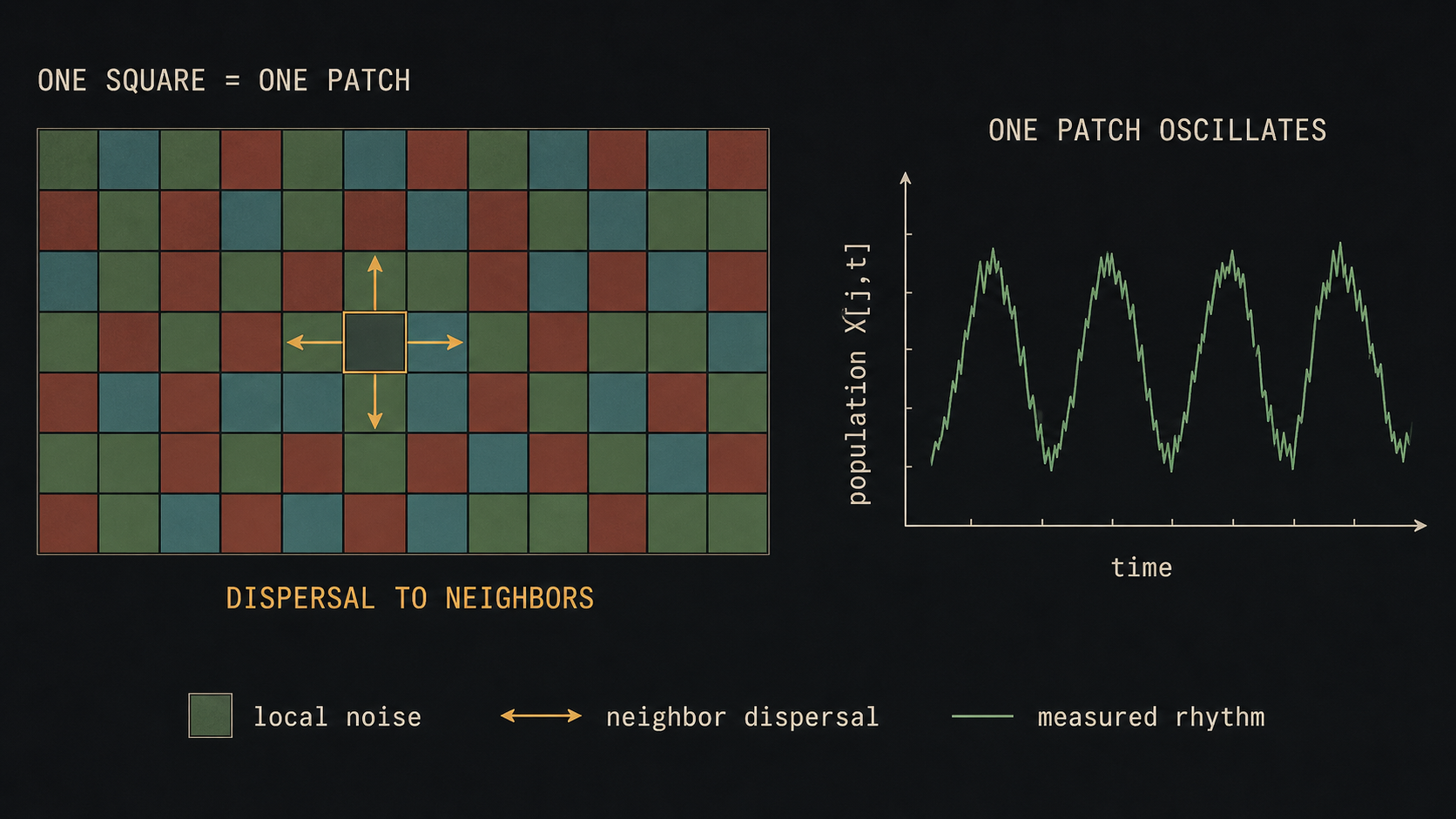 *MODEL IDEA — A lattice view of an ecosystem. One square is one habitat patch. Nearby patches exchange individuals, and each patch can oscillate through high and low population years.*
Noble et al. studied a noisy two-dimensional Ricker map. In that model, each patch follows a population-growth rule that naturally produces a high-low rhythm. Dispersal lets neighboring patches influence each other, while local noise keeps pushing patches apart. Noble's key result was surprising: near the boundary between synchrony and incoherence, this ecological model shows the same large-scale critical fingerprint as the two-dimensional Ising model from physics.
An ecological lattice and a magnet, two completely different systems, can leave the same fingerprint at the edge of order.
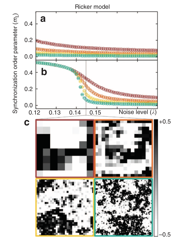 *REFERENCE — Reference from Noble et al. The original work connects local ecological oscillations, noisy spatial coupling, and an Ising-like transition between collective synchrony and incoherence.*
The local noise strength is lambda. Higher lambda means each patch receives stronger independent environmental randomness. The dispersal fraction is epsilon. Higher epsilon means neighboring patches share more individuals. In plain language, lambda pulls patches apart, and epsilon helps nearby patches move together.
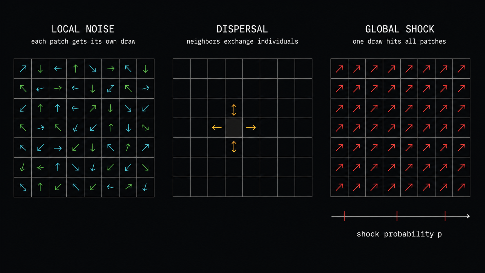 *MODEL INGREDIENTS — Three forces in the model. Local noise is different at every patch, dispersal moves population between neighbors, and the global-shock extension applies one shared environmental draw to the whole lattice.*
The interactive lattice below is a visual toy meant to make the idea feel concrete: many local units update, neighbor structure matters, and the global order trace summarizes whether the grid is moving together or cancelling itself out.
A critical point is the boundary where small changes in noise can create large changes in the whole landscape. Below the boundary, most patches share the same rhythm. Above it, opposite regions cancel each other. Near the boundary, fluctuations are large and spatial patterns can stretch across many patches.
Near criticality, the whole landscape becomes one big amplifier: a small environmental nudge can ripple across many patches at once.
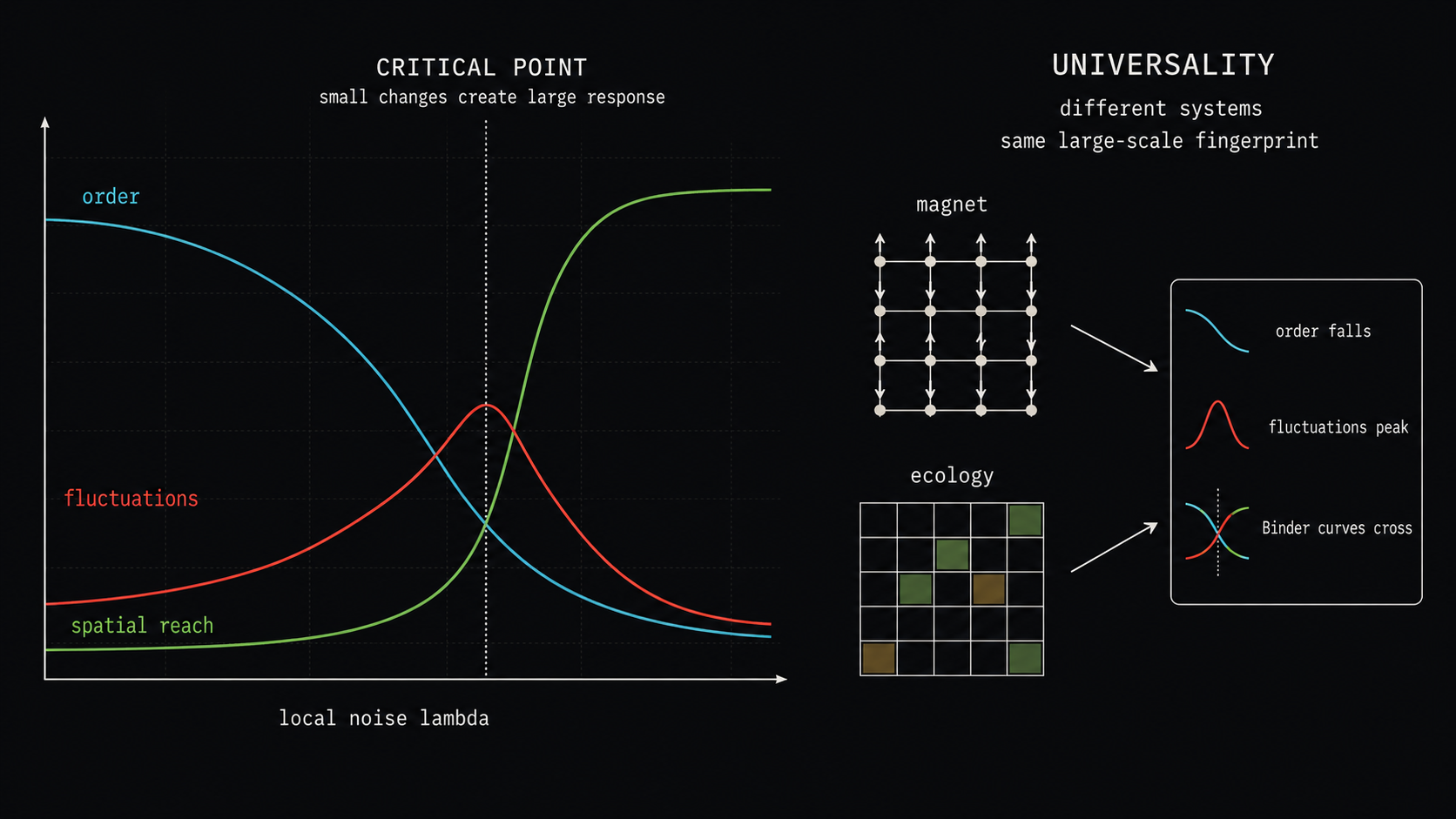 *CONCEPT — Critical behavior and universality in one picture. A magnet and an ecological lattice can have different microscopic rules but still share the same large-scale fingerprint near a transition: order falls, fluctuations peak, and Binder curves cross.*
Every run is reduced to diagnostics. The order parameter m_L measures global agreement. Susceptibility chi_abs measures how strongly that global agreement fluctuates. Binder U_4 is a ratio of moments that gives a stable critical-point crossing across system sizes. The correlation length xi_L measures how far spatial patterns remain connected.
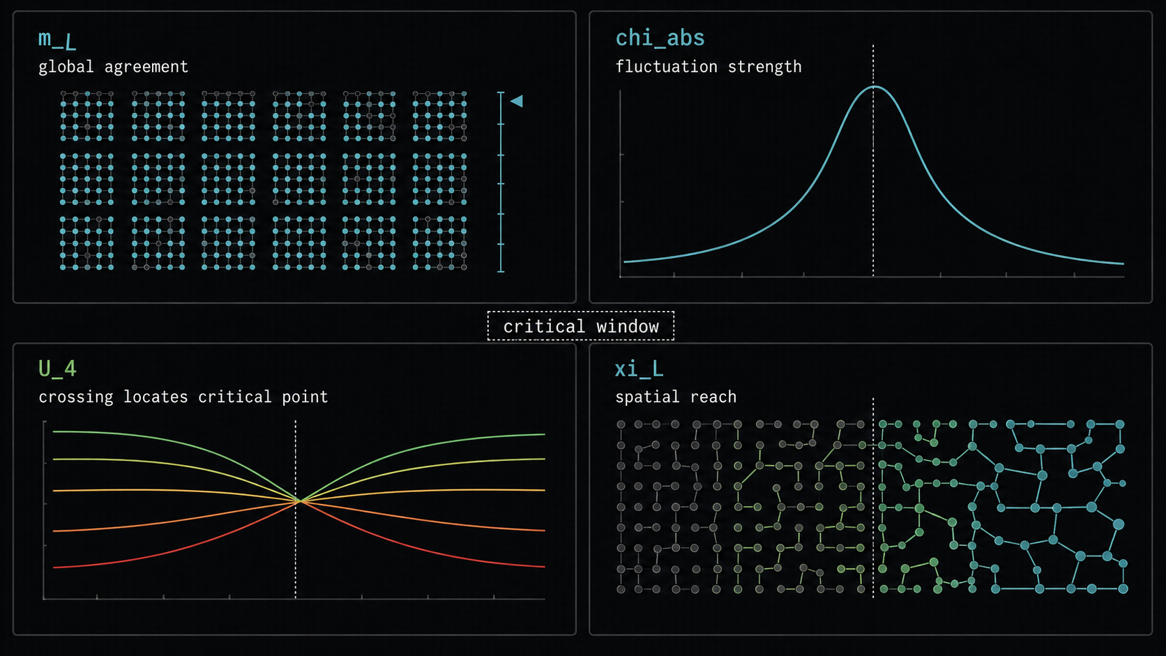 *DIAGNOSTICS — The four main diagnostics used throughout the page. The exact formulas belong in the paper, but the intuition is direct: agreement, fluctuation strength, Binder crossing, and spatial reach.*
```math m_{j,t}=\frac{1}{2}(-1)^{t+1}\left(X_{j,t+1}-X_{j,t}\right),\qquad m_t=\frac{1}{N}\sum_{j=1}^{N}m_{j,t} ``` *The local two-cycle field records which side of the high-low rhythm a patch is on. The spatial average asks whether the full lattice agrees.*
```math m_L=\langle |m_t|\rangle_t,\qquad \chi_{abs}=N\left(\langle m_t^2\rangle_t-\langle |m_t|\rangle_t^2\right) ``` *The order parameter measures agreement. The susceptibility measures how strongly that agreement fluctuates.*
```math U_4=1-\frac{\langle m_t^4\rangle_t}{3\langle m_t^2\rangle_t^2} ``` *Binder U_4 is useful because different lattice sizes cross near the critical point.*
Before adding any new environmental channel, I ran the no-shock control. The parameters are Noble's Ricker baseline: r=2.3, epsilon=0.1, z=4, and p=0. The scan is shorter than Noble's production runs, but it is dense around the critical window and averaged over many random seeds.
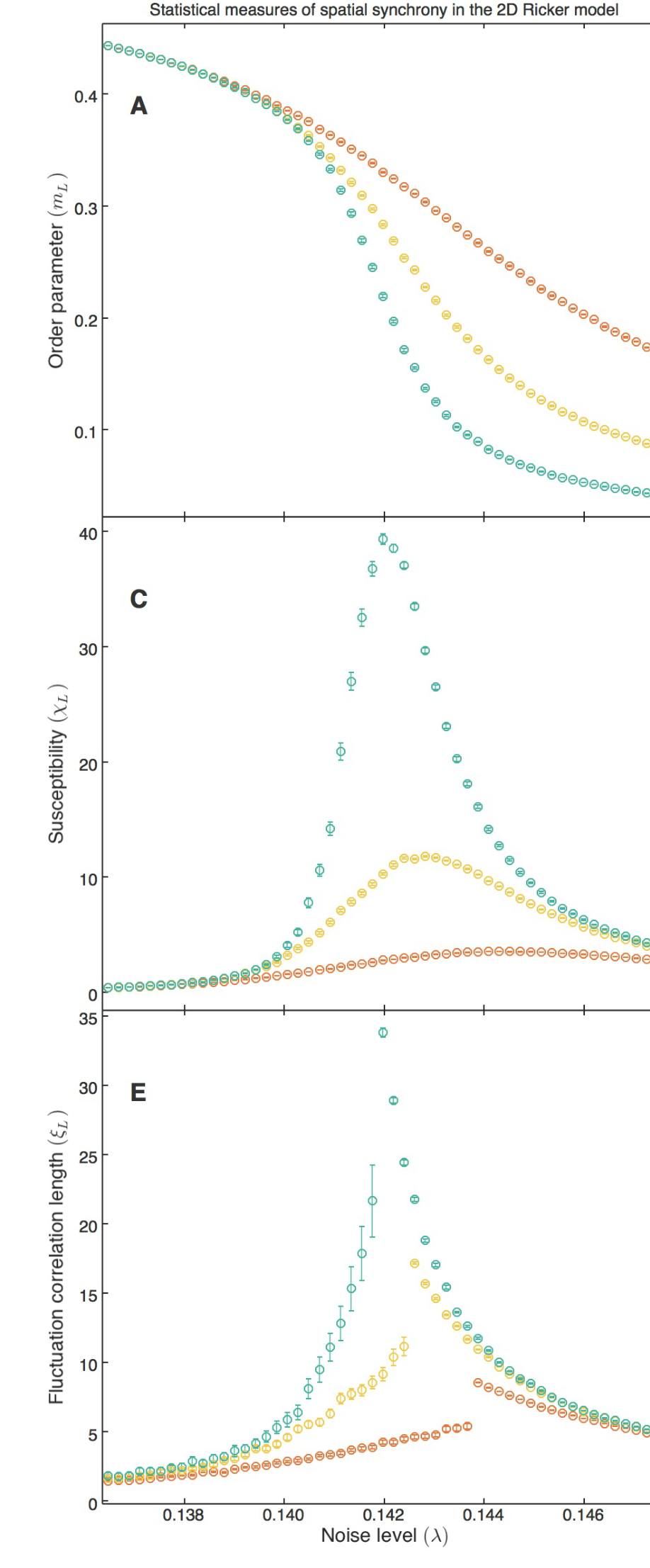 *NOBLE REFERENCE — Noble's reference panels for the Ricker model: order parameter, susceptibility, and fluctuation correlation length as local noise changes.*
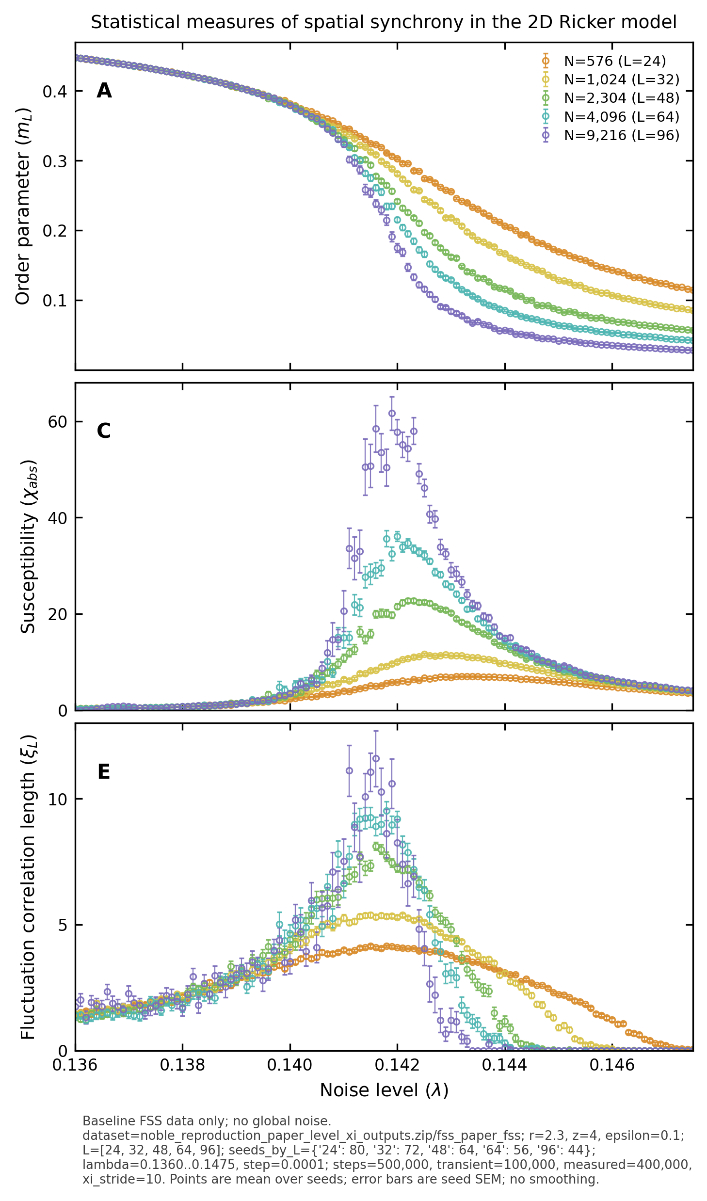 *BASELINE REPRODUCTION — Our no-shock reproduction of the same baseline behavior. The order curve falls, susceptibility peaks in the critical window, and the correlation-length diagnostic rises near the same region.*
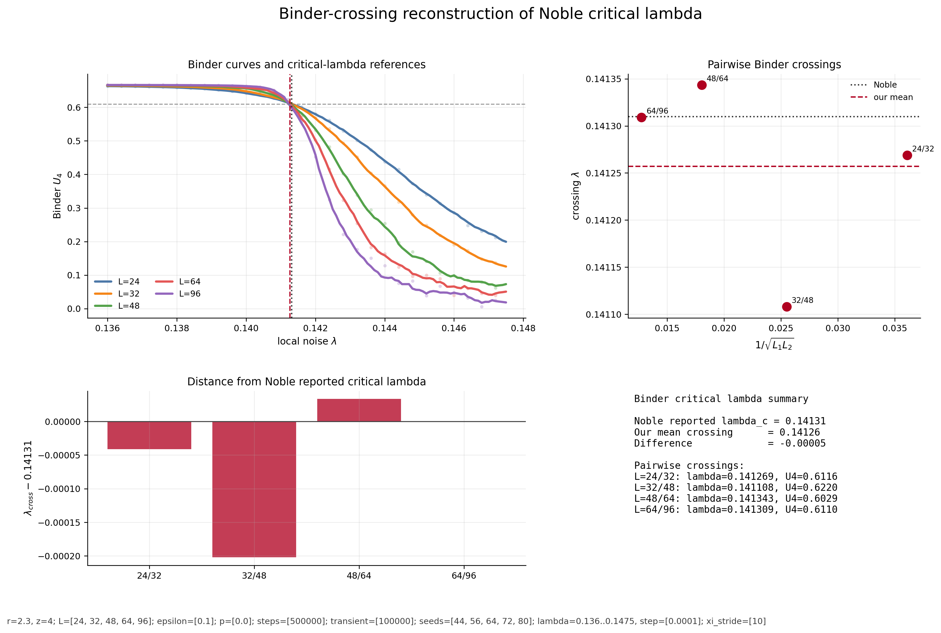 *CRITICAL POINT — Binder crossing for the no-shock baseline. This is the cleanest finite-size estimate of the critical point because it compares moment ratios across lattice sizes instead of relying on one raw peak height.*
Each curve is built from many stochastic runs, not from one lucky simulation. For the baseline reproduction, every parameter block evolves the full lattice for 500,000 steps, discards the first 100,000 steps, and averages the measured diagnostics over seeds. This keeps the page readable while still showing the scale behind the plots.
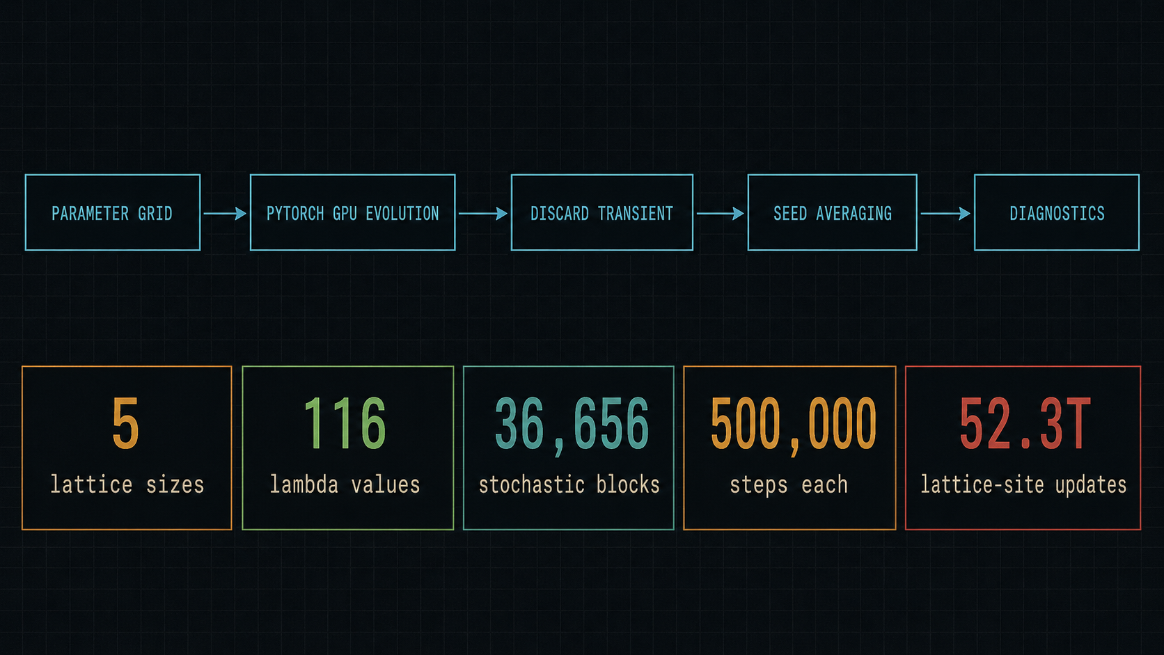 *GPU SWEEP — Baseline simulation scale. The reproduction used dense parameter scans, many stochastic blocks, discarded transients, and GPU tensor updates.*
| Parameter | Baseline value | Why it matters | | --- | --- | --- | | r | 2.3 | growth strength used in Noble's Ricker baseline | | epsilon | 0.1 | nearest-neighbor dispersal fraction | | lambda | 0.136 to 0.1475, step 0.0001 | dense local-noise scan around the critical window | | L | 24, 32, 48, 64, 96 | finite-size check across lattice widths | | steps | 500,000 with 100,000 transient | long enough to estimate post-transient diagnostics | | seeds | 44 to 80 per L | random-seed averaging for smoother curves |
*Baseline scale: 36,656 seed-parameter blocks, 52.3T total lattice-site updates, and 41.9T post-transient measured site updates.*
In the two-dimensional scan, local noise and dispersal act like opposing forces. More local noise makes incoherence easier. More dispersal helps neighboring patches recover agreement. The phase boundary is the curve where those effects balance.
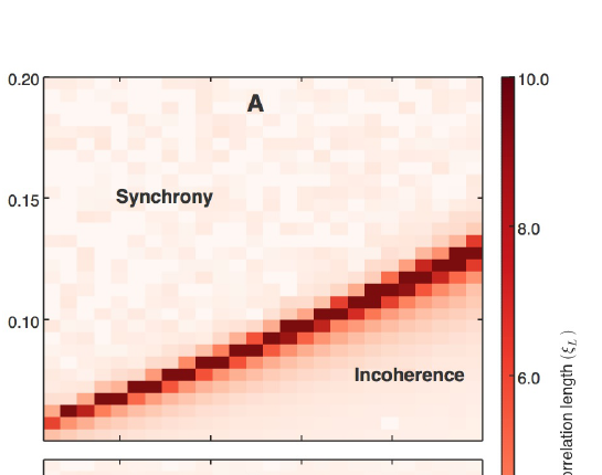 *REFERENCE — Noble's phase-boundary reference for the Ricker model. The high-correlation ridge marks the boundary between collective synchrony and incoherence.*
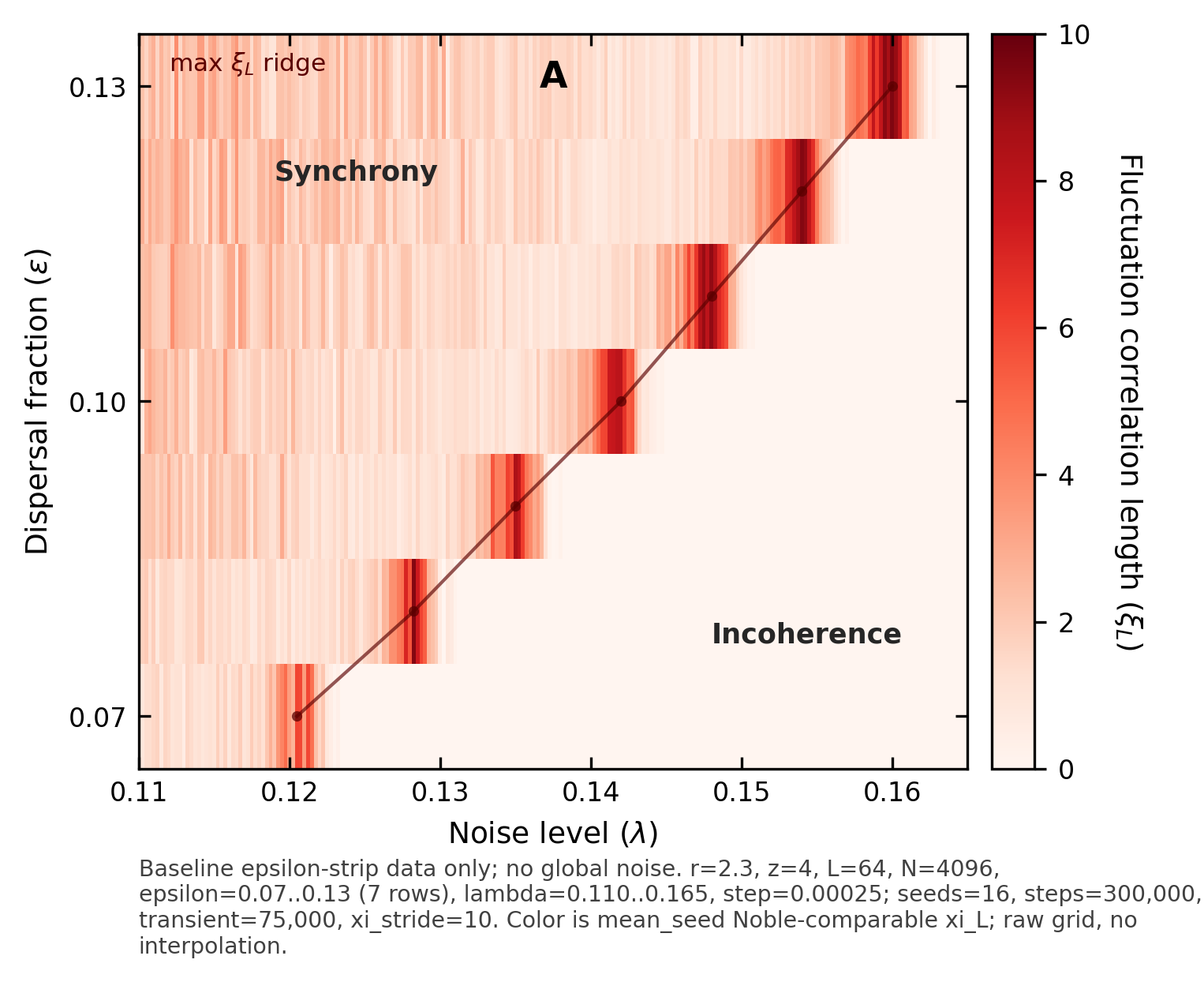 *BASELINE BOUNDARY — Our baseline phase-boundary reconstruction. The important visual pattern is the same: the synchrony boundary moves through the lambda-epsilon plane because dispersal and noise oppose each other.*
Real ecosystems also face shared shocks. A drought, heat wave, regional storm, or resource shock can hit the whole landscape at once. I added that missing channel by sampling one global random value at a time step and applying it to every patch. Rare shock years occur with probability p; when they occur, the shared perturbation is multiplied by a shock multiplier.
When the same drought hits every patch, dispersal does not help anymore: the whole lattice can be pushed in one direction at once.
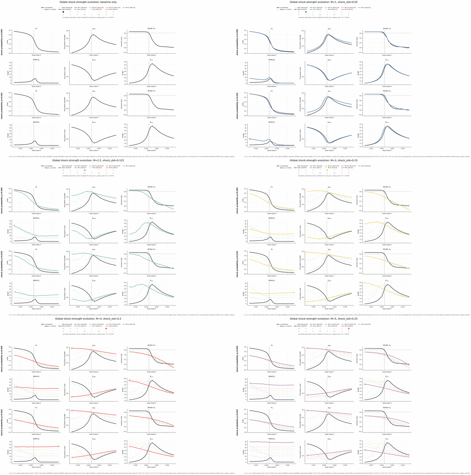 *ANIMATION — Global-noise parameter evolution. The animation shows how the core diagnostics change as shared environmental forcing is varied.*
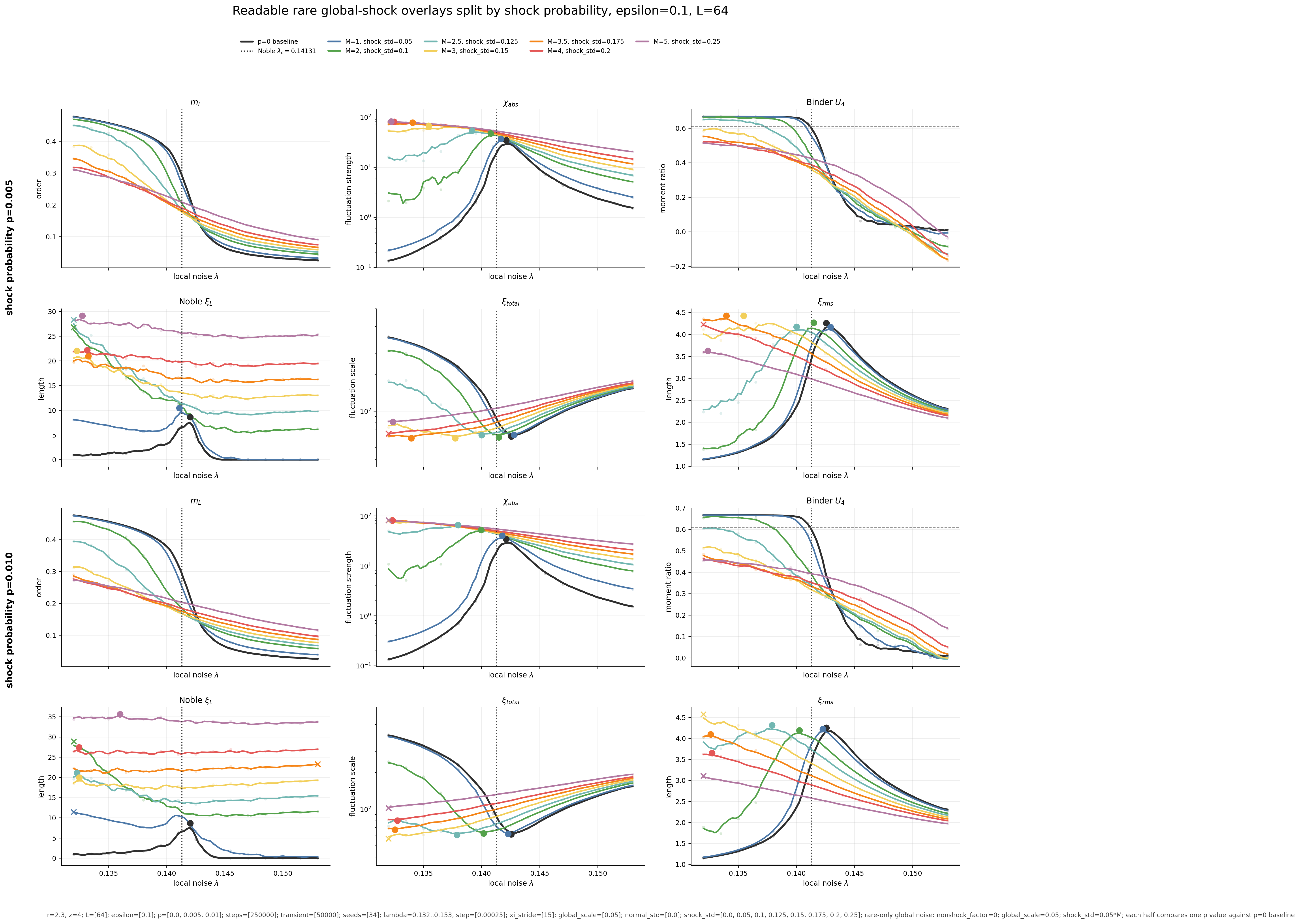 *CALIBRATION — Global-shock calibration. Weak shared perturbations stay close to the no-shock control, while stronger shocks can create a different common-mode regime. That is why the shock extension is reported as a calibration study, not as a finished universality claim.*
The no-shock reproduction is the anchor: it recovers Noble's critical window and Binder crossing with a shorter GPU sweep. The global-noise extension is more delicate. Some settings look like a shifted transition, while stronger shocks can push the whole lattice coherently and create behavior that local noise alone cannot explain.
| Question | Best diagnostic | Current status | | --- | --- | --- | | Did the no-shock model reproduce Noble? | Binder crossing and baseline curves | yes | | Where is the critical point? | Binder U_4 crossing | about lambda_c = 0.14126 | | Does global noise act like local noise? | shock overlays and magnetization traces | not always | | Can strong shocks dominate the lattice? | m_L, chi_abs, xi variants | yes, for some calibrations | | What remains unresolved? | real-space G(r) correlation length | next audit |
*The page intentionally separates the Noble reproduction from the global-shock extension. The first is the validated control. The second is the research extension.*
**Future work:**
**Tools:** Python · PyTorch GPU tensors · NumPy · SciPy · Matplotlib · Monte Carlo sweeps · finite-size scaling · LaTeX